Author: vk5dgr

From mid-August to mid-September, we conducted a Radio Autoencoder (RADAE) test campaign in two phases (a) stored files and (b) a prototype real time system. Ten people joined our test group, with many submitting stored file and real time test results. In particular I would like to thank Mooneer K6AQ, Walter K5WH, Rick W7YC, Yuichi JH0VEQ, Lee BX4ACP, and Simon DJ2LS for posting many useful samples, and for collecting samples of voices other than their own to test.

We are quite pleased with the results, here is a summary:

1. It works well with most speakers, with the exception of one voice tested.  We will look into that issue over the next few months.
2. Some of the samples suggest acquisition issues on certain very long distance channels, but this issue seems to be an outlier, perhaps an area for further work.
3. RADAE works well on high and low SNR channels.  In both cases the speech quality is competitive with SSB.
4. It works on local (groundwave), NVIS, and International DX channels. It works well for (most) males and females, across several languages.
5. Prototype real time/PTT tests suggest it also works well for real time QSOs, no additional problems were encountered compared to the stored files tests. Mooneer will tell you more about that in his September report!

Selected Samples

I estimate we collected around 50 samples, here are just a few that I have selected as good examples. I apologise that I don’t have room to present samples from all our testers, however your work is much appreciated and has contributed greatly to moving this project forward.

Our stored file test system sent SSB and RADAE versions immediately after each other, so the channel is approximately the same. Both SSB and RADAE have the same peak power, and the SSB is compressed to around 6dB Peak to Average Power Ratio (PAPR). In each audio sample below, SSB is presented first.

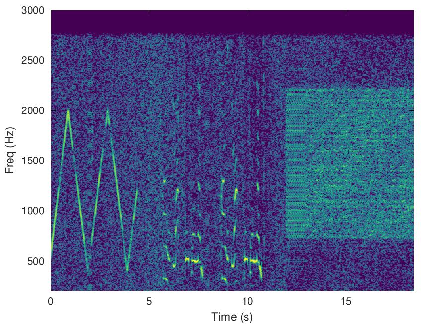
Here is a sample of Joey K5CJ, provided by Rick W7YC. The path is over 13,680km, from Texas, USA to New South Wales, Australia (VK2), on just 25W. Measured SNR was 4dB. Note the fading in the spectrogram, you can hear RADAE lose sync then recover through the fade.

Using another sample of Joey, K5CJ (also at 25W), Rick has provided a novel way to compare the samples:

He writes:

RADAE is in the (R) channel & analog SSB is in the (L) left channel. Listen using stereo speakers, and slide the balance control L-R to hear the impact. Or, listen to it on your smart phone & alternately remove the L & R earbuds – wow. It demonstrates how very well RADAE does over a 13,680 km path!

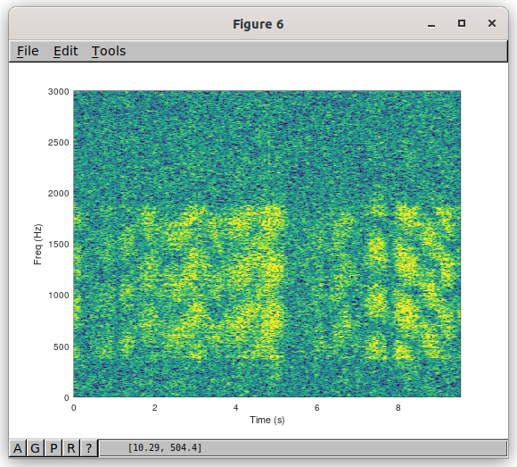
Here is Lee, BX4ACP, sending signals from Taiwan to Thailand in a mixture of English and Chinese using 100W. The measured SNR was 5dB, and frequency selective “barber pole” fading can be seen on the spectrogram.

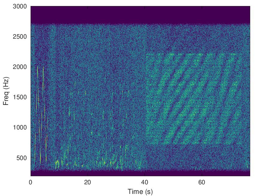
Here is Yuriko (XYL of Yuichi JH0VEQ) using 100W over a 846 km path from Niigata Prefecture to Oita Prefecture in Japan. The reported SNR was just 2dB. From the spectrogram of the RADAE signal, the channel looks quite benign with no obvious fading. However I note the chirp at the start has a few “pieces missing”, which suggests the reported SNR was lower than the SNR experienced by the RADAE signal a few seconds later.

Next Steps for HF RADAE

Encouraged by these results, the FreeDV Project Leadership Team (PLT) has decided to press on with the real time implementation of RADAE, and integration into freedv-gui, so that any ham with a laptop and rig interface can enjoy the mode. This work will take a little time, and involves porting (or linking) some of the Python code to C. Once again, we’ll start with a small test team to get the teething problems worked out before making a general release.

ML Applied to Baseband FM

To date the Radio Autoencoder has been applied to the HF radio channel and OFDM radio architectures. We have obtained impressive results when compared to classical DSP (vocoders + FEC + OFDM modems) and analog (SSB).

A common radio architecture for Land Mobile Radio (LMR) at VHF and UHF is the baseband FM (BBFM) radio, which is used for analog FM, M17, DMR, P25, DStar, C4FM etc. For the digital modes, the bits are converted to baseband pulses (often multi-level) that are fed into an analog FM modulator, passed through the radio channel, and converted back into a sequence of pulses by an analog FM demodulator. Channel impairments include AWGN noise and Rayleigh fading due to vehicle movement. Unlike, HF, low SNR operation is not a major requirement, instead voice quality, spectral occupancy (channel spacing), flat fading, and the use of a patent free vocoder are key concerns.

We have been designing a hybrid machine learning (ML) and DSP system to send high quality voice over the BBFM channel. This is not intended to be a new protocol like those listed above, rather a set of open source building blocks (equivalent to vocoder, modulation and channel coding) that could be employed in a next generation LMR protocol.

It’s early days, but here are some samples from our simulated BBFM system, with an analog FM simulation for comparison.

Original

BBFM, CNR=20dB

BBFM, CNR=20dB, Rayleigh Fading at 60 km/hr

Analog FM, CNR=20dB

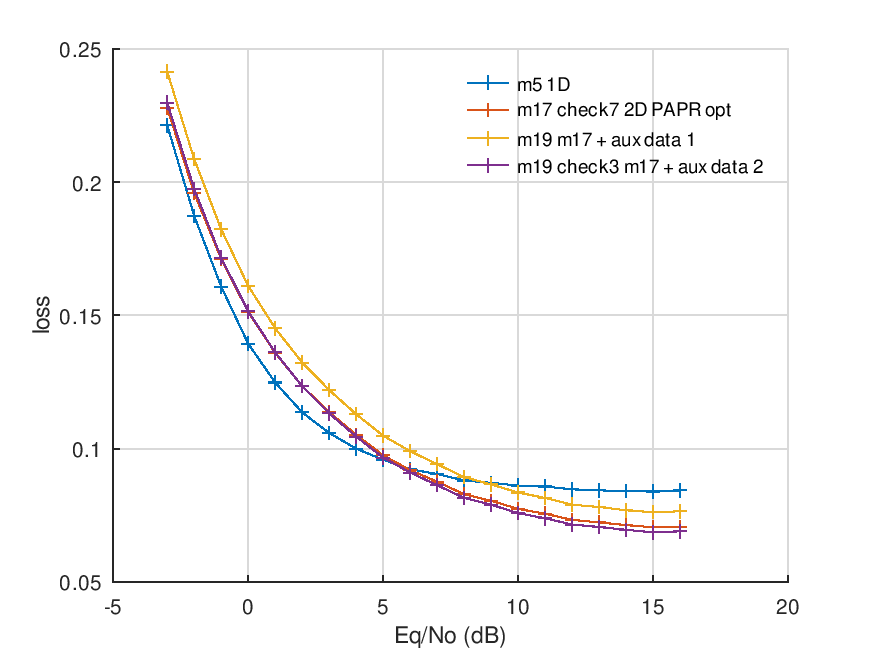
CNR=20dB is equivalent to a Rx level of -107dBm (many LMR contacts operate somewhat above that). The analog FM sample has a 300-3100Hz audio bandwidth, 5kHz deviation, and some Hilbert compression. For the BBFM system we use a pulse train at 2000 symbols/s, that has been trained using a simulation of the BBFM channel. As with HF RADAE, the symbols tend to cluster at +/-1, but are continuously valued. Compared to the HF work, we have ample link margin, which can be traded off for spectral occupancy (channel spacing and adjacent channel interference).

This work is moving quite quickly, so more next month!

Many digital voice systems have the ability to send small amounts of digital data in parallel with the compressed voice. For example in FreeDV we allocate a few bits/frame for call sign and grid square (location) information. This is a bit complex with RADAE, as we don’t actually send any “bits” over the system – it’s all analog PSK symbols.

So I’ve work out a way to inject 25 bits/s of data into the ML network along side the vocoder features. The ML magic spreads these bits across OFDM carriers and appears to do some sort of error protection, as I note the BER is quite low and it show some robustness to multipath. I can tune the bit error rate (BER) by adjusting the loss function and bit rate; a few percent BER at low SNRs (where the voice link falls over) is typical.

The plot below shows the “loss” (RMS error) of the vocoder features as a function of SNR (Energy per symbol/noise density). The vertical axis is the mean square error of the vocoder features through the system – lower is better. It’s useful for comparing networks.

So “red” is model17, which is our control with no auxiliary data. Yellow was my first attempt at injecting data, and purple the final version. You can see purple and red are almost on top of each other, which suggests the vocoder speech quality has barely changed, despite the injection of the data. Something for nothing? Or perhaps this suggests the data bits consume a small amount of power compared the vocoder features.

Much of this month was spent preparing for the August test campaign. I performed a dry run of some over the air (OTA) tests, leading to many tweaks and bug fixes. As usual, I spent a lot of time on making acquisition reliable. Sigh.

The automated tests (ctests) were invaluable, as they show up any effects of tuning one parameter on other system functions. They also let me test in simulation, rather than finding obscure problems through unrepeatable OTA tests. The loss function is a very useful measure for trapping subtle issues. A useful objective measure of speech quality is something I have been missing in many years of speech coding development. It’s sensitive to small errors, and saves a lot of time with listening tests.

I have developed a test procedure for the stored file phase of the August 2024 test campaign. The first phase of testing uses stored files (just like the April test campaign) but this time using the new PAPR optimised waveform and with a chirp header that lets us measure SNR. To make preparation and processing easier, I have developed a web based system for processing the Tx and Rx samples. This means the test team can decode RADAE samples by themselves, without using the command line Linux tools. A test team of about 10 people has been assembled and a few of them have already posted some interesting samples (thanks Yuichi, Simon, and Mooneer).

If you would like to actively participate in RADAE testing, please see this post.

The next phase of testing is real time PTT. The Python code runs in real time, so I have cobbled together a bash script based system (ptt_test.sh) – think of it as crude command line version of freedv-gui. It works OK for me – I can transmit in real time using my IC-7200 to KiwiSDRs, and receive off air from the IC-7200. By using loop back sound devices I can also receive from a KiwSDR. The script only runs on Linux and requires some knowledge of sound cards, but if I can find a few Linux-savvy testers we can use ptt_test.sh to obtain valuable early on-air experience with RADAE. This is an opportunity for someone to make the first live RADAE QSO.

An interesting side project was working with Mooneer to establish the feasibility of running RADAE on ezDV. Unfortunately, this looks unlikely. Modern machine learning systems really require a bit more CPU (like a 1GHz multi-core machine). Fortunately, this sort of CPU is pretty common now (e.g. a Raspberry Pi or cell phone). Once RADAE matures, we will need to reconsider our options for a “headless” adapter type platform.

We are ready to start another test campaign for the radio autoencoder (RADAE). This will consist of stored file tests (like the April campaign), and some real time PTT testing. The draft test procedure is here.

If you would like to join the team testing RADAE, please reach out to us directly or via the comments below.

To use FreeDV with commercial radios we have developed a series of “rig adapters” such as the SM1000 and now ezDV. These are embedded devices that run “headless'”(no GUI) and connect between your SSB radio and a microphone/headset to allow it to run FreeDV.

Our latest prototype speech waveform is RADAE, which is showing promise of improved voice quality and robustness over our existing FreeDV modes and indeed SSB. RADAE uses machine learning (ML) and requires significantly more CPU and memory than existing FreeDV modes.

We would like to know if we can run RADAE on the ezDV, which is based around an ESP32-S3.

The RADAE “stack” consists of the RADAE encoder and decoder, and the FARGAN vocoder. The RADAE encoder and decoder requires around 80 MMAC/s (million multiply-accumulates per second) each, and 1 Mbyte of RAM for the weights. The FARGAN vocoder (used only on receive) requires 1 Mbytes of weights, and around 300 MMAC/s of CPU. The CPU is dominated by the FARGAN vododer, which runs on receive. As the weights are quantised to 8 bits the MMACs can be use 8 bit multiply accumulates, which suits many machines with 8 bit SIMD support.

In practice, you want plenty of overhead, so for a 300 MMACS/s algorithm a machine with above 3x this capability will make the port “easy” (e.g. a recompile with a little SIMD assembly language for the heavy lifting). It also allows you to tweak the algorithm, and run other code on the same machine without worrying about real time issues. If the CPU is struggling you will spent a great deal of time optimizing the code and the algorithm – time that could be better spent elsewhere.

ezDV is based on a ESP32-S3 CPU which has two cores that run at about 240 MHz, has 512 kbytes of local (fast) memory, and 8 MBytes of slower PSRAM that is accessed over a SPI bus. It does have hardware acceleration for integer multiply accumulates.

To answer our question, we developed a simple test program to characterize the ESP32. Many ML operations are “dot products”, or multiplying two vectors together. So we generated a 1Mbyte matrix in PSRAM, and performed a dot product with it one “row” at a time. The other input vector in the dot product was in fast internal memory. The idea was to exercise both the CPU and memory access performance in a way similar to RADAE, but without the hassle of porting the entire algorithm across.

Data type	SIMD?	Raw time (us)	MMACS
int8	No	34887	30
int8	Yes	8490	123
int16	No	47608	22
int16	Yes	16563	63
int16	Yes (using ESP-DSP matrix multiply)	16479	63
int32	No	42689	24

Data type	SIMD?	Raw time (us)	MMACS
int8	No	486	33
int8	Yes	84	195
int16	No	631	25
int16	Yes	98	167
int16	Yes (using ESP-DSP matrix multiply)	88	186
int32	No	419	39

Here is the source code for the program used to measure the ezDV performance.

As shown above, the performance of the matrix multiplication operation on the ESP32-S3 is highly dependent on the size of the matrices involved. For matrices that fit entirely within its internal RAM (either because it can fit within the internal RAM-backed PSRAM cache without many cache misses or because it was originally allocated entirely within internal RAM), performance is fairly reasonable for a micro-controller. In other applications, the ESP32-S3 is able to perform inference on smaller ML models with good performance.

Unfortunately, with larger matrices, the system becomes memory bandwidth limited extremely quickly. For instance, using int16 and ESP-DSP’s matrix multiplication function is slightly more performant than handwritten SIMD assembly when the dataset fits entirely in internal RAM, but are both limited to approximately the same MMACS when the system repeatedly has to go out to PSRAM. int8 using SIMD additionally performs 2x better than int16 because it has to access to PSRAM only half of the time.

These results suggest we will not be able to run the RADAE stack on ezDV. While unfortunate, is it useful to reach this conclusion early so we can consider alternatives for an adapter style implementation of RADAE.

We thought this characterization testing might be useful for others using the ESP32 for ML and other CPU-intense applications, so as part of our open source project philosophy, have written it up here to share.

This post was jointly written by Mooneer and David.

This month I’ve been working on a real time implementation of the Radio Autoencoder (RADAE), suitable for Push To Talk (PTT) use over the air.

One big step was refactoring the core Machine Learning (ML) encoder and decoder to a “stateful” design, that can be run on short (120ms) sequences of data, preserving state each time it is called. The result is a set of command line utilities that can work with streaming audio from a headset or radio. This example demonstrates the full receiver stack: the rx.f32 file (off-air float IQ samples) is decoded to audio samples that are played through your speakers:

cat rx.f32 | python3 radae_rx.py model17/checkpoints/checkpoint_epoch_100.pth -v 1 | ./build/src/lpcnet_demo -fargan-synthesis - - | aplay -f S16_LE -r 16000

I spent some time profiling and with a little optimisation, we now have a real time RADAE Tx and Rx that achieves real time encoding and decoding on Desktop and laptop PCs. Quite surprising given it’s still Python code (with the heavy lifting performed in PyTorch and NumPy). With a little more work, we could use these streaming utilities to build a network based RADAE server, a sound card plug in, or a “headless” RADAE system like the ezDV/SM1000.

Our end goal for a RADAE implementation is a C callable library. While low technical risk, a C port is time consuming, and would delay testing the big unknowns in a new speech communication system such as RADAE. There is also the risk of significant rework of the C code if (when) there are any problems with the waveform. So our priority is to test the RADAE waveform against our requirements, and fortunately the Python version is fast enough for that already.

Over the years we’ve discovered many ways to break digital voice systems. These issues are much easier to fix in simulation so I’ve developed many intricate automated tests, for example tests that simulate slowly varying, stationary channels, and other tests that simulate fast fading like the northern European winter. Do carriers (sine waves) in the middle of a RADAE signal cause it to fall over or make it sync by accident? What happens if the Tx and Rx stations have slightly different sample clock frequencies? I won’t bore you with the details here, but a lot of work goes into this stuff.

While giving RADAE a hard time in simulation I tried the mulitpath disturbed (MPD) channel. This has 2 Hz fading and 4ms delay spread, and is encountered in Winter at high latitudes (e.g. NVIS communications during the UK Winter). It’s tough on HF modems. The mission here is “do not fall over with fast fading” – it’s OK if a few more dB of SNR is required. Here is a sample of what the off air received signal sounds like at 3dB SNR, followed by the decoded audio.

Despite the received signal dipping into the noise at times, RADAE seems to handle it OK. I designed the DSP equalization to handle fast fading, but only trained the ML network with a simulation of 1 Hz fading. So I was concerned the ML might fall over but this time we got lucky! Here is the spectrogram of the same signal – at times the fading completely wipes it out.

One innovation is an “End of Over” system. When a transmission ends, an “end of over” frame is sent and the Rx cleanly “squelches” the receive audio. Previous FreeDV modes would run on for a few seconds making R2D2 sounds, as from the receivers perspective it’s hard to know if the transmitter has finished or you are just in a fade.

On another topic this month I also set up a new WordPress host for this site, and spruced up the content a little. I’m more at home with DSP than SPF and MX records but with the kind support from VentraIP I got there eventually. Thanks Bruce Perens for hosting this site for the last few years.

If you are interested in helping out with the RADAE work I have been building up a list of small chunks of work that need doing using the GitHub Issues system. Many of them require general GitHub/C coding/Linux skills, and not hard core DSP or ML. I’ve listed the skills required in each Issue. Please (please!) discuss them with me first (using the Issue comment system) before kicking off your own PR – I have a really good idea what needs to be done and we need to stay focused.

I have written a test plan for the next phase of over the air (OTA) RADAE testing. The goals will be (a) crowd sourced testing of the latest PAPR-optimised waveform over a variety of channels using the stored file system (b) test real time, PTT conversations over real radio channels using RADAE. This will build our experience and no doubt uncover bugs that will require some rework. I’m on track to start this test campaign in August.

This month I’ve been working on the DSP detail work required for a practical HF waveform based on RADAE. Not as interesting as the Machine Learning (ML) work, but something we need to grind through for a real world HF speech system.

Acquisition

Acquisition is where we determine (a) is a received signal present and (b) if so what is it’s frequency offset and where each frame of “data” starts (coarse timing). The general approach is to search for the pilot symbols at the start of each frame over a grid of time and frequency points. The problem is complicated by the presence of noise, multipath, and high power ML data symbols.

In my earlier FreeDV work I built some ad-hoc acquisition algorithms but this time I took a more mathematical approach. The problem with RADAE is that it operates at very low SNRs which makes acquisition using traditional DSP difficult. Due to the PAPR optimisation the RMS power of the ML data symbols is higher than the classical DSP pilot symbols used for acquisition. While reduced PAPR is in general a good thing, it complicates detection of the pilots.

So I needed a deep dive into the math behind acquisition to get an extra boost in performance. Anyway, the sums showed me two ways I can improve acquisition performance, and it seems to be working well in simulation down to reasonably low SNRs.

Automated Tests

There has been a lot of RADAE code developed over the course of 2024, so much that I’m starting to lose track of it myself. So I’ve added a set of automated tests to make sure everything keeps working and help trap any bugs I might introduce as the code develops. It’s also a neat framework to guide future refactoring and a real time/C port.

Chirp SNR estimator

The April Over the Air (OTA) test campaign showed the need for a way to measure the SNR of off-air samples. It needs to work on HF multipath channels which tend to notch out various frequencies. After a few false starts, I’ve built a “chirp” based SNR estimator. At the start of a transmission, I send a few seconds of chirp signal that sweeps over a range of frequencies. The receiver script knows where this signal is and using a little math can come up with a good estimate of the actual channel SNR.

Interesting Bugs

The previous round of OTA tests was in April. After thinking about the results I found some bugs in the waveform we tested.

I accidentally omitted the cyclic prefix in the waveform tested in April. The cyclic prefix protects us from intersymbol interference, so it “shouldn’t have worked” on HF channels. Exploring just why it worked (and worked rather well) is on the TODO list, and might explain the poor performance on DX channels (e.g Japan to Australia). Sometimes accidents lead to “light bulb” moments.

Another possible bug is the use of fixed timing estimate used for the entire 10 second sample (we don’t adjust timing after the initial estimate). The ionosphere is changing all the time, and the Tx DAC and Rx ADC sample clocks are also slightly different which means a timing estimate that varies over time. So a fixed timing estimate is a bad idea, and I was kind of lucky it worked on most of the samples we collected.

Recent Progress and OTA Low PAPR Tests

So I figure the last few months of work is probably enough for this round of development:

• Two new low PAPR waveforms (750 and 1500Hz RF bandwidth)
• Acquisition system improvements
• Addressing some bugs from the April 2024 test campaign
• Chirp based SNR measurement to calibrate our OTA tests

While there are many possibilities for further development, I don’t want to go too far down any R&D rabbit holes without checking against real world performance. So I’m preparing for some more stored file OTA tests, to see how we are performing against our stated goals of low and high SNR performance that is competitive with SSB.

Here are some initial samples (using a sample of my voice) of the 1500Hz low PAPR waveform (model17) over a 2000km path at 14.250 MHz, at a few watts transmit power:

The SNR is measured from the chirp. The chirp signal has 0dB PAPR, so this is the SNR at the peak power of the SSB and RADAE signals. The RMS power and hence average SNR of the SSB signal would be about 6dB lower (-5.5dB), and the RADAE about 0.8dB lower (-0.3 dB). So with the same power amplifier, RADAE delivers about 5dB more power to the receiver than SSB.

An hour or so later I turned up the power to get a high SNR sample over the same 2000km path:

While much easier to understand, even at high SNR there is quite a bit of background noise with SSB (this could possibly be improved with DSP noise reduction). However there is some “vocoder” distortion on the RADAE signal as well – it’s not totally clean. You actually have to listen fairly carefully to hear differences between the low and high SNR RADAE samples. This might mean we’ve biased the training towards “low SNR”, rather than “highest quality”. These results also suggests we can run 1.5W rather than 100W, for similar speech quality, as 10log10(100/1.5) = 18dB.

While performing these test I noticed a bunch of little things to look into:

• A pop artifact in one of my samples that goes away when the input speech level changes. Suggests the ML is entering territory is hasn’t seen in training.
• I’m not sure if my Tx power from my SSB radio is staying constant as intended with a low PAPR waveform – need to sample the actual Tx power and plot on the spec-an. I need to confirm all three signals are at the same peak power.
• The high SNR RADAE speech quality isn’t consistent across samples, some speakers sound a bit better. This is subjective of course so needs a further look.

Tx Spurious

At high SNRs there is some out of band spurious Tx energy (e.g. from 2000 to 3000 Hz) in the in the PAPR optimised RADAE signal. We should remove this if possible.

Next Steps

Every time I put this technology over real radio channels I learn a lot and have a bunch more questions and tasks added to my TODO list. However I do feel it’s time to focus on building a real time system that we can test with real PTT conversations. Even a rudimentary system that has some teething problems will teach us a lot. We have several ML models we can try (e.g. high and low PAPR, 750 and 1500 Hz wide waveforms), and it’s quite easy to try others as our experience improves.

So I will continue working towards a real time implementation so we can get on the air and test this technology with real time PTT conversations. Some challenges ahead are (a) a state machine sync system that can acquire and determine when an over is complete (b) refactoring the code to run on modem frame size chunks rather than several seconds of samples (c) some way for anyone to run RADAE in real time (either in Python or a C port) with streaming audio (d) other chunks of DSP like tracking frequency, amplitude, and timing offsets as they evolve (e) a way to perform controlled tests and evaluate quality automatically – subjective reports and ad-hoc testing is not very reliable.

The last few months have been focused on building up the DSP code required to try the Radio Auto-encoder (RADAE) over the air. In order to answer the big question of “does it really work” as quickly as possible, I had to skim over many intriguing topics. So now that we have a qualified “yes” to the big question – I’ve returned to some Machine Learning (ML) R&D to explore a some intriguing ideas:

• Reduction of the “latent dimension” and hence RF bandwidth of the RADAE signal.
• Encouraging the network to train 2 dimensional constellations rather than 1D.
• Training for low Peak to Average Power Ratio (PAPR) – a potential 6dB improvement.

To date RADAE has used a “latent dimension” of 80 symbols every 40ms, which are mapped to 20 OFDM carriers at 50 symbols/s, resulting in a RF bandwidth of 1000 Hz. I spent some time exploring how to to reduce this to dimension 40, i.e. a 10 carrier, 500 Hz bandwidth signal. This would result in more efficient use of spectrum. With fewer carriers our pilot based equalization work better as there would be more power per pilot symbol. Fewer carriers also helps reduce PAPR. On the negative side, classical communications theory predicts a narrower bandwidth signal will perform worse on HF channels, and may be less power efficient (e.g. BER performance of 8PSK versus QPSK).

The original RADAE design has a one dimensional bottleneck that limits the amplitude of real valued symbols to +/-1. Given additive noise, the network would always place constellation points at +/-1 in order to minimize the effect of noise. As the dimension reduced, distortion increased as there was nowhere in 1D space to place additional constellation points without being unduly affected by noise. I reasoned that encouraging the network to train two dimensional constellations would help. For example in classical digital systems, we can use an 8PSK constellation, each point is equal distance away from the origin. If the SNR is high enough, this can send more information per symbol than QPSK.

So I arranged the elements of the latent vector in complex number pairs (e.g. 20 complex valued symbols for a 40 element latent vector), and set up a two dimensional bottleneck that constrained the magnitude of the complex symbols trained by the network. This worked, I can now obtain good performance from a dimension 40 system. Curiously, the resulting constellations are circles, rather than discrete points.

Also this month I developed a method for comparing ML models objectively. The method runs the training database through a trained model at a range of SNRs, and produces curves of model “loss against Eq/No” for the model (Eq is the energy of one PSK symbol). I feel there is a reasonable match between these curves and the subjective speech quality. Having an objective method of measuring a models performance lets me know if I’m on the right track with a ML model design without tedious listening tests.

OK, so now we have an objective measure for comparing models, a way of training lower dimensional models, and some understanding of 2D constellations: i.e. how to train them, and what to expect from the 2D constellations developed by training.

Using these tools, I attempted to build a PAPR optimised ML model. I estimate a low PAPR waveform has the potential to provide a further 6dB improvement at the receiver compared to a classical DSP OFDM waveform – so this is definitely worth exploring. This requires a “time domain” 2D bottleneck that simulates the way a power amplifier saturates. Combining this with multipath training is tricky, and I have tried several different approaches. At the time of writing I believe I have a way forward with a hybrid time-frequency domain model, and am currently evaluating the results. The design uses OFDM and classical DSP for equalisation, and ML for PAPR optimisation, and achieves a PAPR of less than 1 dB.

Here are some samples that show the PAPR optimised waveform over a simulated multipath poor (MPP) fast fading channel. They both have the same “peak power to noise” P/No ratio. Imagine them both being transmitted from the same radio with 100W peak power, over the same (really bad) HF radio channel, to the same receiver.

Note the difference in the receiver SNR. The “S” in S/N is the RMS power at the receiver, which is lower for SSB as the SSB PAPR is higher (around 6dB, after compression). The goal of most radio systems is to maximise the RMS power at the receiver. So with the same transmitter, we have achieved around 6dB higher SNR at the Rx by carefully minimising the PAPR of the RADAE waveform.

Here are the spectrograms, note the model18 dim 40 RADAE signal uses only about 750 Hz of RF bandwidth (500 Hz for the ML PSK symbols plus some bandwidth for OFDM overheads). The moth-eaten effect is the multipath channel wiping out chunks of the signal.

There are many other areas we could explore, but as we don’t have infinite time, I’m choosing to time box the ML R&D before we lock in a V1.0 design, and proceed to real time implementation.

Next month I will round out the ML design work, address a few other bugs, and attempt to arrive at a RADAE design suitable for our first real time implementation.

The Right to Innovate in the HF Data Space

On the HF data front, I’ve been working with Simon DJ2LS to test and merge several libcodec2 PRs to support FreeDATA. This work has improved protocol efficiency and enabled Simon to “homebrew” his own custom OFDM waveforms. His first attempt at a new waveform has roughly doubled the highest data transfer speed of FreeDATA. Simon is working on a new FreeDATA release that includes these improvements. We also have a 16QAM prototype waveform under development, which in high SNR channels, will double the speed again.

One of the PRs supports custom configuration of the OFDM modem, for example you can plug in the number of carriers, symbol rate, and number of bits per frame at “init time” without writing any C code. Empowering Hams (and indeed anyone) to build their own HF data waveforms is important. This work “preserves the right to innovate” in the HF data space, a key value of the ARDC.

This month I took a vacation, so less work that usual on FreeDV. I traveled by road from my home in Adelaide to Western Australia (WA), reaching the South-Western tip of Australia, about 3000km away. South Western WA is a lovely part of the country, and the trip included the adventure of crossing the 1200km Nullarbor plane (translated: no trees).

But back to the business of HF digital voice. Given the encouraging results from our initial Radio Autoencoder (RADAE) over the air (OTA) tests, we have expanded our program of testing to include Hams from different countries. It takes a lot of work to develop a new speech communication system , so it’s important to validate the design as early as possible. Much smarter to do this in the current simulation form, rather than put in ten times the work on a real time implementation, release it, and find out it falls over in a common use case. This is experience talking – we’ve learned many lessons after a decade of FreeDV development.

So we are testing the prototype RADAE design using crowd sourcing. I have approached several Hams for help in testing RADAE signals over their local radio channels and in different languages. They provide me with a 10s speech sample in their language, I send them back a file of RADAE samples that they can transmit over the air. The received RADAE signal is recorded off air by them (e.g. using a KiwiSDR), we then decode and evaluate. This is all done in non real time using stored files being emailed back and forth.

In particular I would like to thank Kanda JH0PCF, Yuichi JH0VEQ, and Simon DJ2LS for your help. Some take aways:

1. RADAE works well in Japanese and German, as well as English.
   It handles Near Vertical Incidence Skywave (NVIS) channels quite well. This is typical of local (several hundred km) HF communication in countries like Japan and the UK. The signal goes straight up and straight down.
2. However on the samples tested so far, RADAE is falling over with long distance (e.g. Japan to Australia) communications, so some more work required there.
3. The speech quality is competitive with SSB at high and low SNRs, however we need a better way to measure the actual SNR of off air signals to “calibrate” the results. So I need to hit the math on that one to develop a suitable algorithm.

Some comments from the test team:

I listened to the voice that was replied. RADAE has no problem with Japanese demodulation. In fact, I feel that RADAE’s demodulated audio is easier to hear than SSB. I thought the sound quality was close to the 2020 mode implemented in the current version. It’s a strange feeling to be able to experience FM mode quality audio with SSB. (Kanda, JH0PCF)

It feels, if we can hear SSB clearly, then RADAE also works, but as soon as we are coming closer to the edge of ability of hearing SSB, also RADAE struggles. But the radae output is really nice, much better voice output compared to SSB. Using your last example, I first thought, you’ve send me the default audio example (ie source sample), so yes, its really nice. (Simon, DJ2LS)

Here is a example from Kanda at low SNR

Kanda JH0PCF, 20W, received by Tokyo KiwiSDR (RADAE)

The two signals are transmitted one after the other, so get (more or less) the same channel conditions. The spectrogram below shows (left to right) the sine wave tone, SSB, then RADAE. Note about half the RADAE signal is wiped out at the start, but it seems to sound OK.

Here’s a medium SNR (8dB-ish) sample from Simon, DJ2LS, over a 1100km path at about 10W peak (1-2W RMS):

Yuichi performed a couple of novel experiments that I hadn’t thought of. Here is RADAE compared to existing FreeDV modes, transmitted a few seconds apart, so over more or less the same channel at roughly the same power. SNRs are around 8dB.

Unfortunately 2020B didn’t sync on this channel/SNR. I feel the 700E sample could possibly be improved (e.g. levels, microphone, filtering), but it does illustrate the problems with current FreeDV modes – the speech quality borders on the lower level required for communication and it can be a struggle to get consistent results. This is something we have recognized and are attempting to address with our ARDC funded R&D program.

As a fairer comparison, here is the sample used for RADAE testing passed through a FreeDV 700E simulation with no channel errors:

Project Plan Pivot

Given the encouraging results with RADAE, we’ve pivoted our ARDC project plan to focus on RADAE, and have paused development of Codec 2 and FreeDV modes. RADAE appears to be our strongest candidate for satisfying the top three goals we set for ourselves when applying for the ARDC grant:

1. Improve speech quality to a level comparable to commercial codecs.
2. Develop a “rag chew” FreeDV mode with subjective speech quality comparable to SSB at high SNRs.
3. Improve low SNR operation such that FreeDV is superior to SSB over poor HF channels.

We are on track to meet (and indeed exceed) the first two goals, but I think the final goal has yet to be demonstrated (e.g. SSB and the current incarnation of RADAE fall over at roughly the same SNR). There are a few bugs and many practical issues to work through before we have a real world version of RADAE that anyone can use. Plus there will be a few “gotchas” we haven’t thought of yet. Plenty for me to do in the coming months!

I’ve also been working on HF data modem software with Simon from the FreeDATA project. In next months report we hope to present a new FreeDATA release incorporating this work, resulting in a significant boost in FreeDATA performance.

This month was spent building up the “classical” DSP support code around the Radio Autoencoder, so I could test it over the air using real radio signals. Can we repeat the impressive low SNR results from simulation over real radio channels? This meant coding up an OFDM modem in PyTorch, lots of testing, and a bunch of support scripts to drive the radio hardware.

The algorithms we developed last year on improving FreeDV acquisition and designing filters came in handy, especially at the low SNRs required for this work.

The first test was “over the cable” (OTC) at VHF (144.5 MHz) using a HackRF transmitter, switchable attenuator as the “channel”, and a RTLSDR as the receiver. The noise (N) is injected by the physical properties (noise figure) of the RTLSDR receiver, so the S/N is controllable by the level (S) presented by the switchable attenuator. My calculations indicated it should work around the -135dBm level, and sure enough it did – sounding just like the simulations (see Feb 2024 for examples). This was a great confidence boost as it’s hard to argue with real world noise, but easy to mess up the calibration of noise simulated by software.

For comparison a narrow band FM signal will fall over at around -120dBm, and a first generation digital VHF radio (using proprietary speech codecs) perhaps a few dB lower. Although to be fair the digital VHF systems also transmit ancillary digital data at the same time, which consumes some of their power and bandwidth.

Next step was HF radio, a somewhat tougher channel. This required quite a bit more work on the OFDM sync algorithms, but eventually I was ready to transmit a signal using my HF radio. I sent a 5W signal over a 500km HF path to a KiwiSDR, and passed the received signal through the Radio Autoencoder system. Much to my surprise, it worked first time! Good quality audio over several different paths and channel types, up to 2000 km away. It seems quite robust to the channels I have tested so far, including NVIS, EMI corrupted receivers, and SNRs below 0dB.

These are encouraging results for the Radio Autoencoder. I’m now pondering next steps. I think it makes sense to test the system with some more samples and over different channels. Also, at some point we need a C port so this can be used in real time by anyone.

FreeDATA Update

Part of our ARDC grant activities is to support the FreeDATA project. Simon and team have recently completed a major re-write and FreeDATA is back on the air. This month I’ve been working with Simon on a faster modem waveform for “ACK” packets, that will help speed up the FreeDATA protocol. I’m also pleased to see FreeDATA working over real HF channels, including this 7 hour 1.44Mbyte file transfer over an 800km path.

This month I’ve been working on a feasibility study using an autoencoder derived from RDOVAE [1], based on code originally written by Jean Marc Valin and Jan Büthe for an Opus application. The goal is to see if we can send good quality speech over HF multipath channels at low SNRs.

The autoencoder takes as input a typical set of vocoder features (short term spectrum, pitch, voicing), then applies time based prediction and transforms to arrive at a small number of parameters that can be sent over a channel. This is similar to an old school vocoder that uses classical DSP, except Machine Learning (ML) allows us to learn non-linear transforms and prediction, which tend to be more powerful.

Usually, after the transformation/prediction stage we then quantise to a low bit rate, then use Forward Error Correction (FEC) and modems to send the bits over a channel. However this latest work takes a novel twist – we train the autoencoder to generate PSK symbols that we send over the channel. It effectively combines quantisation, channel coding, and modulation. The symbols tend to cluster around +/-1 like BPSK but are continuously valued. So it’s like a discrete time, continuously valued (analog) PSK.

This month I’ve been building up the code required to test the idea over multipath (HF) channels. This mean reshaping the PSK symbols into an OFDM modem frame, and adding a multipath simulation. The initial results are encouraging, with speech quality better than any existing FreeDV mode, and competitive with SSB at low SNRs. At high SNRs the quality is also quite good, better than analog FM.

However this is all early days. To expedite answering the key questions, the current simulation ignores a lot of real world issues like acquisition, phase, frequency and timing offset correction. I reasoned that we have classical DSP solutions to these problems that work pretty well, so instead I focused on multipath performance as experience has shown that is the toughest issue with HF digital speech.

The ML code used for training includes a channel model. As an experiment, I added a saturating HF power amplifier model. The output was an OFDM modem waveform with a 1dB Peak to Average Power Ratio (PAPR), which is an excellent result. Our FreeDV waveforms run at around 4.5 dB, and SSB with a good compressor 4-6dB.

ML systems tend to work well until they experience conditions outside what they have been trained for. So I’m taking small steps, and planning to test a variety of channel impairments one by one, looking for that “ML gotcha”. I’m also spending way to much time checking my channel model calculations – handling the shift from digital PSK to analog has taken some careful thought and is a bit mind bending after 35 years of work in digital PSK!

The next step is to build up acquisition and synchronization code, and get to a point where we can send and receive signals over real RF channels. I’ll start with an Over The Cable (OTC) test on the bench, and work up to the point where we can play stored files over real HF channels.

[1] J.-M. Valin, J. Büthe, A. Mustafa, Low-Bitrate Redundancy Coding of Speech Using a Rate-Distortion-Optimized Variational Autoencoder, Proceedings of International Conference on Acoustics, Speech, and Signal Processing (ICASSP), 2023.